Differential Equations of Special Kinds

Differential Equations

Introduction

First-Order Differential Equations

Directly Integrable Equations
  Motion of a Body - Problem 1
  Motion of a Body - Problem 2
  Motion of a Body - Problem 3
  The Spontaneous Radioactive of Substance

Separable Equations
  Motion of Particals in Viscous Fluid
  Newton's Model of Cooling
  Model of Population

Homogeneous Equations

Linear Equations

Bernoulli Equations

Exact Differential Equations

Differential Equations of Higher Orders

Basic Conceptions
Equations of Special Kinds

Some Graphic Illustrations using MATLAB

Clich here to go to

Clich here to go to Definite Inegrals

Some Graphic Illustrations using MATLAB

Real-Life Problems: Motion of a Body - Problem 1 » Motion of a Body - Problem 2 » Motion of a Body - Problem 3 » The Spontaneous Radioactive of Substance » Motion of Particals in Viscous Fluid » Newton's Model of Cooling » Model of Population

The main purpose of this section is to illustrate graphically the solutions to a differential equation, using a computer algebra system and technical computing environment such as MATLAB that in combination with analytical calculations gives the best way of using differential equations in the mathematical modeling and interpretation of real-world phenomena. Let us consider an initial value problem relative to the following differential equation of the second order, involving two arbitrary parameters, a and b:

The solution depends on a correlation between the parameters. By making use of the below MATLAB command we obtain the sequence of windows containing the graphical representations of solutions:

     clear
     clf
     b=1; a = 2*b;
     y = dsolve('D2y + a*Dy + b*y = 0', 'y(0) = 1', 'Dy(0) = 0', 'x')
     subplot(221)
     ezplot(y, [0,20])
     title('y`` + a y` + b y = 0, y(0) = 1, y`(0) = 0')
     ylabel('y'),
     legend('a > b')
     grid
     pause

     a = b;
     y = dsolve('D2y + a*Dy + b*y = 0', 'y(0) = 1', 'Dy(0) = 0', 'x')
     subplot(222)
     ezplot(y, [0,20])
     title('')
     ylabel('y'),
     legend('a = b')
     grid
     pause <>br
     a = 1/8 * b;
     y = dsolve('D2y + a*Dy + b*y = 0', 'y(0) = 1', 'Dy(0) = 0', 'x')
     subplot(223)
     ezplot(y, [0,20])
     title('')
     ylabel('y'),
     legend('a < b')
     grid
     pause

     a =0;
     y = dsolve('D2y + a*Dy + b*y = 0', 'y(0) = 1', 'Dy(0) = 0', 'x')
     subplot(224)
     ezplot(y, [0,20])
     title('')
     ylabel('y'),
     legend('a = b')
     grid

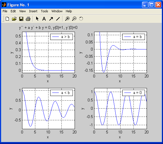
MATLAB produces the following solutions, correspondingly:
    1.    y = exp(-x)+exp(-x)*x
    2.    y = exp(-1/2*x)*cos(1/2*3^(1/2)*x)+1/3*3^(1/2)*exp(-1/2*x)*sin(1/2*3^(1/2)*x)
    3.    y = 1/255 * 255^(1/2) * exp(-1/16 * x) * sin(1/16 * 255^(1/2) * x) + exp(-1/16 * x) * cos(1/16 * 255^(1/2) * x)
    4.    y = cos(x)

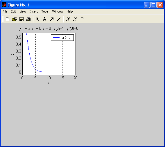
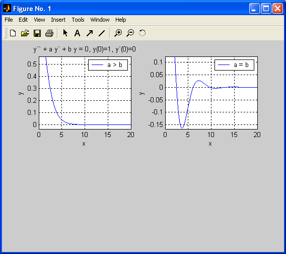
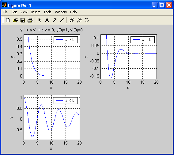
In each case, the solution differs from the others in a qualitative relation.
Case (1) corresponds to a damping process while in case (2) the solution gives quickly damped oscillations.
In case (3) we deals with slowly decreasing oscillations - in comparison with case (2).
Case (4) corresponds to harmonic oscillations.